A Practical Guide to Object Detection using the Popular YOLO Framework – Part III (with Python codes)

Introduction

How easy would our life be if we simply took an already designed framework, executed it, and got the desired result? Minimum effort, maximum reward. Isn’t that what we strive for in any profession?

I feel incredibly lucky to be part of our machine learning community where even the top tech behemoths embrace open source technology. Of course it’s important to understand and grasp concepts before implementing them, but it’s always helpful when the ground work has been laid for you by top industry data scientists and researchers.

This is especially true for deep learning domains like computer vision. Not everyone has the computational resources to build a DL model from scratch. That’s where predefined frameworks and pretained models come in handy. And in this article, we will look at one such framework for object detection – YOLO. It’s a supremely fast and accurate framework, as we’ll see soon.

So far in our series of posts detailing object detection (links below), we’ve seen the various algorithms that are used, and how we can detect objects in an image and predict bounding boxes using algorithms of the R-CNN family. We have also looked at the implementation of Faster-RCNN in Python.

In part 3 here, we will learn what makes YOLO tick, why you should use it over other object detection algorithms, and the different techniques used by YOLO. Once we have understood the concept thoroughly, we will then implement it it in Python. It’s the ideal guide to gain invaluable knowledge and then apply it in a practical hands-on manner.

I highly recommend going through the first two parts before diving into this guide:

• A Step-by-Step Introduction to the Basic Object Detection Algorithms (Part 1)
• A Practical Implementation of the Faster R-CNN Algorithm for Object Detection (Part 2)

 

Table of Contents

1. What is YOLO and Why is it Useful?
2. How does the YOLO Framework Function?
3. How to Encode Bounding Boxes?
4. Intersection over Union and Non-Max Suppression
5. Anchor Boxes
6. Combining all the Above Ideas
7. Implementing YOLO in Python

 

What is YOLO and Why is it Useful?

The R-CNN family of techniques we saw in Part 1 primarily use regions to localize the objects within the image. The network does not look at the entire image, only at the parts of the images which have a higher chance of containing an object.

The YOLO framework (You Only Look Once) on the other hand, deals with object detection in a different way. It takes the entire image in a single instance and predicts the bounding box coordinates and class probabilities for these boxes. The biggest advantage of using YOLO is its superb speed – it’s incredibly fast and can process 45 frames per second. YOLO also understands generalized object representation.

This is one of the best algorithms for object detection and has shown a comparatively similar performance to the R-CNN algorithms. In the upcoming sections, we will learn about different techniques used in YOLO algorithm. The following explanations are inspired by Andrew NG’s course on Object Detection which helped me a lot in understanding the working of YOLO.

 

How does the YOLO Framework Function?

Now that we have grasp on why YOLO is such a useful framework, let’s jump into how it actually works. In this section, I have mentioned the steps followed by YOLO for detecting objects in a given image.

• YOLO first takes an input image:

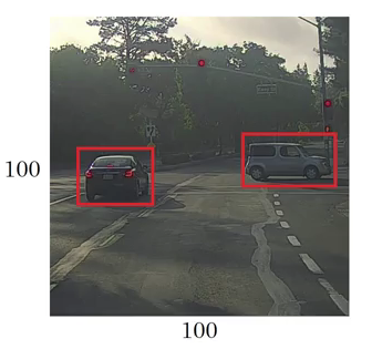
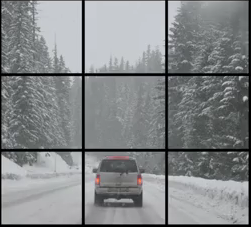
• The framework then divides the input image into grids (say a 3 X 3 grid):

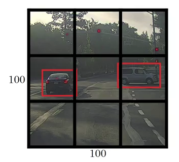
• Image classification and localization are applied on each grid. YOLO then predicts the bounding boxes and their corresponding class probabilities for objects (if any are found, of course).

Pretty straightforward, isn’t it? Let’s break down each step to get a more granular understanding of what we just learned.

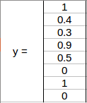
We need to pass the labelled data to the model in order to train it. Suppose we have divided the image into a grid of size 3 X 3 and there are a total of 3 classes which we want the objects to be classified into. Let’s say the classes are Pedestrian, Car, and Motorcycle respectively. So, for each grid cell, the label y will be an eight dimensional vector:

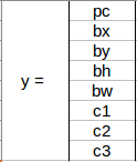
Here,

• pc defines whether an object is present in the grid or not (it is the probability)
• bx, by, bh, bw specify the bounding box if there is an object
• c1, c2, c3 represent the classes. So, if the object is a car, c2 will be 1 and c1 & c3 will be 0, and so on

Let’s say we select the first grid from the above example:

Since there is no object in this grid, pc will be zero and the y label for this grid will be:

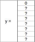
Here, ‘?’ means that it doesn’t matter what bx, by, bh, bw, c1, c2, and c3 contain as there is no object in the grid. Let’s take another grid in which we have a car (c2 = 1):

Before we write the y label for this grid, it’s important to first understand how YOLO decides whether there actually is an object in the grid. In the above image, there are two objects (two cars), so YOLO will take the mid-point of these two objects and these objects will be assigned to the grid which contains the mid-point of these objects. The y label for the centre left grid with the car will be:

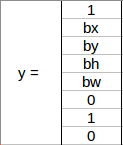
Since there is an object in this grid, pc will be equal to 1. bx, by, bh, bw will be calculated relative to the particular grid cell we are dealing with. Since car is the second class, c2 = 1 and c1 and c3 = 0. So, for each of the 9 grids, we will have an eight dimensional output vector. This output will have a shape of 3 X 3 X 8.

So now we have an input image and it’s corresponding target vector. Using the above example (input image – 100 X 100 X 3, output – 3 X 3 X 8), our model will be trained as follows:

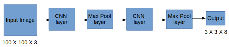
We will run both forward and backward propagation to train our model. During the testing phase, we pass an image to the model and run forward propagation until we get an output y. In order to keep things simple, I have explained this using a 3 X 3 grid here, but generally in real-world scenarios we take larger grids (perhaps 19 X 19).

Even if an object spans out to more than one grid, it will only be assigned to a single grid in which its mid-point is located. We can reduce the chances of multiple objects appearing in the same grid cell by increasing the more number of grids (19 X 19, for example).

 

How to Encode Bounding Boxes?

As I mentioned earlier, bx, by, bh, and bw are calculated relative to the grid cell we are dealing with. Let’s understand this concept with an example. Consider the center-right grid which contains a car:

So, bx, by, bh, and bw will be calculated relative to this grid only. The y label for this grid will be:

pc = 1 since there is an object in this grid and since it is a car, c2 = 1. Now, let’s see how to decide bx, by, bh, and bw. In YOLO, the coordinates assigned to all the grids are:

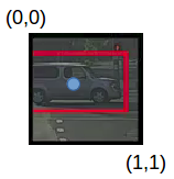
bx, by are the x and y coordinates of the midpoint of the object with respect to this grid. In this case, it will be (around) bx = 0.4 and by = 0.3:

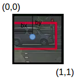
bh is the ratio of the height of the bounding box (red box in the above example) to the height of the corresponding grid cell, which in our case is around 0.9. So,  bh = 0.9. bw is the ratio of the width of the bounding box to the width of the grid cell. So, bw = 0.5 (approximately). The y label for this grid will be:

Notice here that bx and by will always range between 0 and 1 as the midpoint will always lie within the grid. Whereas bh and bw can be more than 1 in case the dimensions of the bounding box are more than the dimension of the grid.

In the next section, we will look at more ideas that can potentially help us in making this algorithm’s performance even better.

 

Intersection over Union and Non-Max Suppression

Here’s some food for thought – how can we decide whether the predicted bounding box is giving us a good outcome (or a bad one)? This is where Intersection over Union comes into the picture. It calculates the intersection over union of the actual bounding box and the predicted bonding box. Consider the actual and predicted bounding boxes for a car as shown below:

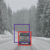
Here, the red box is the actual bounding box and the blue box is the predicted one. How can we decide whether it is a good prediction or not? IoU, or Intersection over Union, will calculate the area of the intersection over union of these two boxes. That area will be:

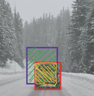
IoU = Area of the intersection / Area of the union, i.e.

IoU = Area of yellow box / Area of green box

If IoU is greater than 0.5, we can say that the prediction is good enough. 0.5 is an arbitrary threshold we have taken here, but it can be changed according to your specific problem. Intuitively, the more you increase the threshold, the better the predictions become.

There is one more technique that can improve the output of YOLO significantly – Non-Max Suppression.

One of the most common problems with object detection algorithms is that rather than detecting an object just once, they might detect it multiple times. Consider the below image:

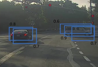
Here, the cars are identified more than once. The Non-Max Suppression technique cleans up this up so that we get only a single detection per object. Let’s see how this approach works.

1. It first looks at the probabilities associated with each detection and takes the largest one. In the above image, 0.9 is the highest probability, so the box with 0.9 probability will be selected first:

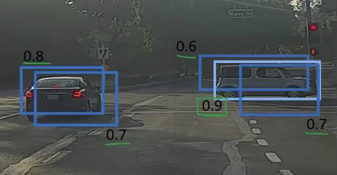
2. Now, it looks at all the other boxes in the image. The boxes which have high IoU with the current box are suppressed. So, the boxes with 0.6 and 0.7 probabilities will be suppressed in our example:

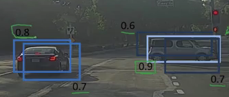
3. After the boxes have been suppressed, it selects the next box from all the boxes with the highest probability, which is 0.8 in our case:

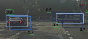
4. Again it will look at the IoU of this box with the remaining boxes and compress the boxes with a high IoU:

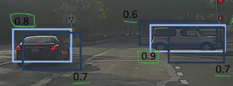
5. We repeat these steps until all the boxes have either been selected or compressed and we get the final bounding boxes:

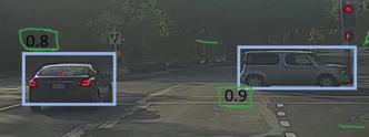
This is what Non-Max Suppression is all about. We are taking the boxes with maximum probability and suppressing the close-by boxes with non-max probabilities. Let’s quickly summarize the points which we’ve seen in this section about the Non-Max suppression algorithm:

1. Discard all the boxes having probabilities less than or equal to a pre-defined threshold (say, 0.5)
2. For the remaining boxes:
   1. Pick the box with the highest probability and take that as the output prediction
   2. Discard any other box which has IoU greater than the threshold with the output box from the above step
3. Repeat step 2 until all the boxes are either taken as the output prediction or discarded

There is another method we can use to improve the perform of a YOLO algorithm – let’s check it out!

 

Anchor Boxes

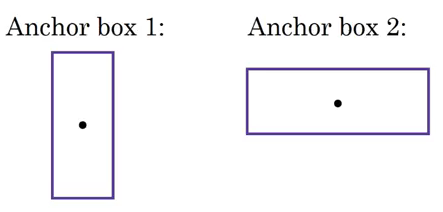
We have seen that each grid can only identify one object. But what if there are multiple objects in a single grid? That can so often be the case in reality. And that leads us to the concept of anchor boxes. Consider the following image, divided into a 3 X 3 grid:

Remember how we assigned an object to a grid? We took the midpoint of the object and based on its location, assigned the object to the corresponding grid. In the above example, the midpoint of both the objects lies in the same grid. This is how the actual bounding boxes for the objects will be:

We will only be getting one of the two boxes, either for the car or for the person. But if we use anchor boxes, we might be able to output both boxes! How do we go about doing this? First, we pre-define two different shapes called anchor boxes or anchor box shapes. Now, for each grid, instead of having one output, we will have two outputs. We can always increase the number of anchor boxes as well. I have taken two here to make the concept easy to understand:

This is how the y label for YOLO without anchor boxes looks like:

What do you think the y label will be if we have 2 anchor boxes? I want you to take a moment to ponder this before reading further. Got it? The y label will be:

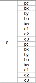
The first 8 rows belong to anchor box 1 and the remaining 8 belongs to anchor box 2. The objects are assigned to the anchor boxes based on the similarity of the bounding boxes and the anchor box shape. Since the shape of anchor box 1 is similar to the bounding box for the person, the latter will be assigned to anchor box 1 and the car will be assigned to anchor box 2. The output in this case, instead of 3 X 3 X 8 (using a 3 X 3 grid and 3 classes), will be 3 X 3 X 16 (since we are using 2 anchors).

So, for each grid, we can detect two or more objects based on the number of anchors. Let’s combine all the ideas we have covered so far and integrate them into the YOLO framework.

 

Combining the Ideas

In this section, we will first see how a YOLO model is trained and then how the predictions can be made for a new and previously unseen image.

 

Training

The input for training our model will obviously be images and their corresponding y labels. Let’s see an image and make its y label:

Consider the scenario where we are using a 3 X 3 grid with two anchors per grid, and there are 3 different object classes. So the corresponding y labels will have a shape of 3 X 3 X 16. Now, suppose if we use 5 anchor boxes per grid and the number of classes has been increased to 5. So the target will be 3 X 3 X 10 X 5 = 3 X 3 X 50. This is how the training process is done – taking an image of a particular shape and mapping it with a 3 X 3 X 16 target (this may change as per the grid size, number of anchor boxes and the number of classes).

 

Testing

The new image will be divided into the same number of grids which we have chosen during the training period. For each grid, the model will predict an output of shape 3 X 3 X 16 (assuming this is the shape of the target during training time). The 16 values in this prediction will be in the same format as that of the training label. The first 8 values will correspond to anchor box 1, where the first value will be the probability of an object in that grid. Values 2-5 will be the bounding box coordinates for that object, and the last three values will tell us which class the object belongs to. The next 8 values will be for anchor box 2 and in the same format, i.e., first the probability, then the bounding box coordinates, and finally the classes.

Finally, the Non-Max Suppression technique will be applied on the predicted boxes to obtain a single prediction per object.

That brings us to the end of the theoretical aspect of understanding how the YOLO algorithm works, starting from training the model and then generating prediction boxes for the objects. Below are the exact dimensions and steps that the YOLO algorithm follows:

• Takes an input image of shape (608, 608, 3)
• Passes this image to a convolutional neural network (CNN), which returns a (19, 19, 5, 85) dimensional output
• The last two dimensions of the above output are flattened to get an output volume of (19, 19, 425):
  • Here, each cell of a 19 X 19 grid returns 425 numbers
  • 425 = 5 * 85, where 5 is the number of anchor boxes per grid
  • 85 = 5 + 80, where 5 is (pc, bx, by, bh, bw) and 80 is the number of classes we want to detect
• Finally, we do the IoU and Non-Max Suppression to avoid selecting overlapping boxes

 

Implementing YOLO in Python

Time to fire up our Jupyter notebooks (or your preferred IDE) and finally implement our learning in the form of code! This is what we have been building up to so far, so let’s get the ball rolling.

The code we’ll see in this section for implementing YOLO has been taken from Andrew NG’s GitHub repository on Deep Learning. You will also need to download the pretrained weights required to run this code.

Let’s first define the functions that will help us choose the boxes above a certain threshold, find the IoU, and apply Non-Max Suppression on them. Before everything else however, we’ll first import the required libraries:

import os
import matplotlib.pyplot as plt
from matplotlib.pyplot import imshow
import scipy.io
import scipy.misc
import numpy as np
import pandas as pd
import PIL
import tensorflow as tf
from skimage.transform import resize
from keras import backend as K
from keras.layers import Input, Lambda, Conv2D
from keras.models import load_model, Model
from yolo_utils import read_classes, read_anchors, generate_colors, preprocess_image, draw_boxes, scale_boxes
from yad2k.models.keras_yolo import yolo_head, yolo_boxes_to_corners, preprocess_true_boxes, yolo_loss, yolo_body

%matplotlib inline

Now, let’s create a function for filtering the boxes based on their probabilities and threshold:

def yolo_filter_boxes(box_confidence, boxes, box_class_probs, threshold = .6):
    box_scores = box_confidence*box_class_probs
    box_classes = K.argmax(box_scores,-1)
    box_class_scores = K.max(box_scores,-1)
    filtering_mask = box_class_scores>threshold
    scores = tf.boolean_mask(box_class_scores,filtering_mask)
    boxes = tf.boolean_mask(boxes,filtering_mask)
    classes = tf.boolean_mask(box_classes,filtering_mask)
 
    return scores, boxes, classes

Next, we will define a function to calculate the IoU between two boxes:

def iou(box1, box2):
    xi1 = max(box1[0],box2[0])
    yi1 = max(box1[1],box2[1])
    xi2 = min(box1[2],box2[2])
    yi2 = min(box1[3],box2[3])
    inter_area = (yi2-yi1)*(xi2-xi1)
    box1_area = (box1[3]-box1[1])*(box1[2]-box1[0])
    box2_area = (box2[3]-box2[1])*(box2[2]-box2[0])
    union_area = box1_area+box2_area-inter_area
    iou = inter_area/union_area
 
    return iou

Let’s define a function for Non-Max Suppression:

def yolo_non_max_suppression(scores, boxes, classes, max_boxes = 10, iou_threshold = 0.5):
    max_boxes_tensor = K.variable(max_boxes, dtype='int32')
    K.get_session().run(tf.variables_initializer([max_boxes_tensor]))
    nms_indices = tf.image.non_max_suppression(boxes,scores,max_boxes,iou_threshold)
    scores = K.gather(scores,nms_indices)
    boxes = K.gather(boxes,nms_indices)
    classes = K.gather(classes,nms_indices)

    return scores, boxes, classes

We now have the functions that will calculate the IoU and perform Non-Max Suppression. We get the output from the CNN of shape (19,19,5,85). So, we will create a random volume of shape (19,19,5,85) and then predict the bounding boxes:

yolo_outputs = (tf.random_normal([19, 19, 5, 1], mean=1, stddev=4, seed = 1),
                   tf.random_normal([19, 19, 5, 2], mean=1, stddev=4, seed = 1),
                   tf.random_normal([19, 19, 5, 2], mean=1, stddev=4, seed = 1),
                   tf.random_normal([19, 19, 5, 80], mean=1, stddev=4, seed = 1))

Finally, we will define a function which will take the outputs of a CNN as input and return the suppressed boxes:

def yolo_eval(yolo_outputs, image_shape = (720., 1280.), max_boxes=10, score_threshold=.6, iou_threshold=.5):
    box_confidence, box_xy, box_wh, box_class_probs = yolo_outputs
    boxes = yolo_boxes_to_corners(box_xy, box_wh)
    scores, boxes, classes = yolo_filter_boxes(box_confidence, boxes, box_class_probs, threshold = score_threshold)
    boxes = scale_boxes(boxes, image_shape)
    scores, boxes, classes = yolo_non_max_suppression(scores, boxes, classes, max_boxes, iou_threshold)

    return scores, boxes, classes

Let’s see how we can use the yolo_eval function to make predictions for a random volume which we created above:

scores, boxes, classes = yolo_eval(yolo_outputs)

How does the outlook look?

with tf.Session() as test_b:
    print("scores[2] = " + str(scores[2].eval()))
    print("boxes[2] = " + str(boxes[2].eval()))
    print("classes[2] = " + str(classes[2].eval()))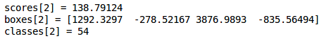

‘scores’ represents how likely the object will be present in the volume. ‘boxes’ returns the (x1, y1, x2, y2) coordinates for the detected objects. ‘classes’ is the class of the identified object.

Now, let’s use a pretrained YOLO algorithm on new images and see how it works:

sess = K.get_session()
class_names = read_classes("model_data/coco_classes.txt")
anchors = read_anchors("model_data/yolo_anchors.txt")

yolo_model = load_model("model_data/yolo.h5")

After loading the classes and the pretrained model, let’s use the functions defined above to get the yolo_outputs.

yolo_outputs = yolo_head(yolo_model.output, anchors, len(class_names))

Now, we will define a function to predict the bounding boxes and save the images with these bounding boxes included:

def predict(sess, image_file):
    image, image_data = preprocess_image("images/" + image_file, model_image_size = (608, 608))
    out_scores, out_boxes, out_classes = sess.run([scores, boxes, classes], feed_dict={yolo_model.input: image_data, K.learning_phase(): 0})

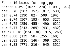
    print('Found {} boxes for {}'.format(len(out_boxes), image_file))

    # Generate colors for drawing bounding boxes.
    colors = generate_colors(class_names)

    # Draw bounding boxes on the image file
    draw_boxes(image, out_scores, out_boxes, out_classes, class_names, colors)

    # Save the predicted bounding box on the image
    image.save(os.path.join("out", image_file), quality=90)

    # Display the results in the notebook
    output_image = scipy.misc.imread(os.path.join("out", image_file))

    plt.figure(figsize=(12,12))
    imshow(output_image)

    return out_scores, out_boxes, out_classes

Next, we will read an image and make predictions using the predict function:

img = plt.imread('images/img.jpg')
image_shape = float(img.shape[0]), float(img.shape[1])
scores, boxes, classes = yolo_eval(yolo_outputs, image_shape)

Finally, let’s plot the predictions:

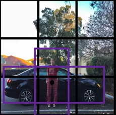
out_scores, out_boxes, out_classes = predict(sess, "img.jpg")

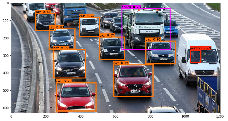
Not bad! I especially like that the model correctly picked up the person in the mini-van as well.

 

End Notes

Here’s a brief summary of what we covered and implemented in this guide:

• YOLO is a state-of-the-art object detection algorithm that is incredibly fast and accurate
• We send an input image to a CNN which outputs a 19 X 19 X 5 X 85 dimension volume.
• Here, the grid size is 19 X 19 and each grid contains 5 boxes
• We filter through all the boxes using Non-Max Suppression, keep only the accurate boxes, and also eliminate overlapping boxes

YOLO is one of my all-time favorite frameworks and I’m sure you’ll see why once you implement the code on your own machine. It’s a great way of getting your hands dirty with a popular computer vision algorithm.