Fast R-CNN for object detection

With the technological advancements and increase in computational power that we have seen since 2014 when the R-CNN paper was published, it is easy for us to now see the obvious pitfalls of R-CNNs the authors discovered back then:

• Multi-stage, expensive training: The separate training processes required for all the stages of the network — fine-tuning a CNN on object proposals, learning an SVM to classify the feature vector of each proposal from the CNN and learning a bounding box regressor to fine-tune the object proposals proves to be a burden in terms of time, computation and resources. For example, to train the SVM, we would need the features of thousands of possible region proposals to be written to the disk from the previous stage.
• Slow test time: Given this multi-stage pipeline, detection using a simple VGG network as the backbone CNN takes 47s/image.

Another paper published in 2015, SPP-Nets or “Spatial Pyramid Pooling Networks”[3] solved one part of the problem. Its main contribution was a) the use of multi-scale pooling of image features to improve the network performance for classification and detection and also b) the use of arbitrary sized input images to train CNN’s despite the use of fully connected (FC) layers. In its detection pipeline, it introduced an important concept— extracting a single feature map from the entire image only once, and pooling the features of arbitrary sized “region proposals” for that image, from this single feature map. This allowed their network to run orders of magnitude faster than R-CNN. Instead of running a CNN on 2000 region proposals from an image individually like R-CNN, they have only one forward pass from which they can pool the features of all 2000 candidate proposals.

Fast R-CNN Pipeline

Architecture details:

To better understand how and why the Fast R-CNN improved efficiency and performance of R-CNN and SPP Networks, let’s first look into its architecture.

• The Fast R-CNN consists of a CNN (usually pre-trained on the ImageNet classification task) with its final pooling layer replaced by an “ROI pooling” layer and its final FC layer is replaced by two branches — a (K + 1) category softmax layer branch and a category-specific bounding box regression branch.

Figure 1: The Fast R-CNN pipeline

Figure 2: The ROI pooling layer as a special case of SPP layer

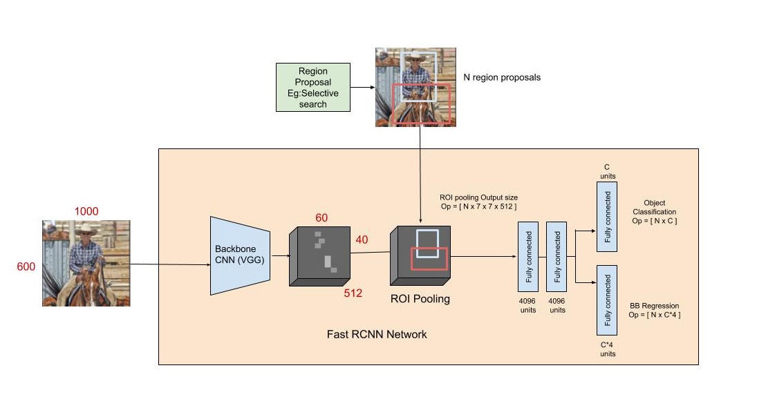
• The entire image is fed into the backbone CNN and the features from the last convolution layer are obtained. Depending on the backbone CNN used, the output feature maps are much smaller than the original image size. This depends on the stride of the backbone CNN, which is usually 16 in the case of a VGG backbone.
• Meanwhile, the object proposal windows are obtained from a region proposal algorithm like selective search[4]. As explained in Regions with CNNs, object proposals are rectangular regions on the image that signify the presence of an object.
• The portion of the backbone feature map that belongs to this window is then fed into the ROI Pooling layer.
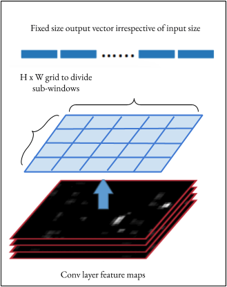
• The ROI pooling layer is a special case of the spatial pyramid pooling (SPP) layer with just one pyramid level. The layer basically divides the features from the selected proposal windows (that come from the region proposal algorithm) into sub-windows of size h/H by w/W and performs a pooling operation in each of these sub-windows. This gives rise to fixed-size output features of size (H x W) irrespective of the input size. H and W are chosen such that the output is compatible with the network’s first fully-connected layer. The chosen values of H and W in the Fast R-CNN paper is 7. Like regular pooling, ROI pooling is carried out in every channel individually.
• The output features from the ROI Pooling layer (N x 7 x 7 x 512 where N is the number of proposals) are then fed into the successive FC layers, and the softmax and BB-regression branches. The softmax classification branch produces probability values of each ROI belonging to K categories and one catch-all background category. The BB regression branch output is used to make the bounding boxes from the region proposal algorithm more precise.

Loss:

The classification branch of the softmax layer gives probabilities for every ROI over (K +1) categories p = p₀, … pₖ. The classification loss L𝒸ₗₛ(p,u) is given by -log(pᵤ) which is the log loss for the true class u.

Equation 1: smooth L1 loss for BB regression

Equation 2: Joint loss for multi-task training

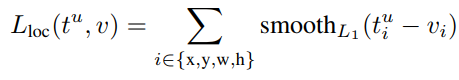
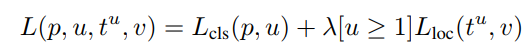
The regression branch produces 4 bounding box regression offsets tᵏᵢ where i = x, y, w, and h. (x, y) stands for the top-left corner and w and h denote the height and width of the bounding box. The true bounding box regression targets for a class u are indicated by vᵢ where i = x, y, w, and h when u≥1. The case where u=0 is ignored because the background classes have no groundtruth boxes. The regression loss used is a smooth L1 loss given in equation 1. The joint multi-task loss for each ROI is given by the combination of the two losses as shown in equation 2. Notice that the Fast R-CNN here has a combined learning scheme that fine-tunes the backbone CNN, and classifies and regresses the bounding box.

Training:

• During training, each mini-batch is constructed from N=2 images. The mini-batch consists of 64 ROIs from each image.
• Like R-CNN, 25% of the ROIs are object proposals that have at least 0.5 IoU with a ground-truth bounding box of a foreground class. These would be positive for that particular class and would be labelled with the appropriate u=1…K.
• The remaining ROIs are sampled from proposals that have an IoU with groundtruth bounding boxes between [0.1, 0.5). These ROIs are labelled as belonging to the class u = 0 (background class).
• Until before the ROI pooling layer, the entire image goes through the CNN. This way, all the ROIs from the same image share computation and memory in the forward and backward passes through the CNN (before the ROI pooling layer).
• The sampling strategy (sampling all the ROI in a batch from very few images) allows the entire module — feature generation, classification, and regression — to be trained together, unlike SPP Nets. In the SPP Nets most of the input ROIs come from different images, so the training process for detection only finetunes the fully connected layers after the feature generation because it is not feasible to update the weights before the SPP layer (some of the ROI’s could have very large receptive fields on the original image). The actual features still come from a pre-trained network that was trained for classification. This limits the accuracy of SPP Nets.
• Note that the batch size of the network is very small for the CNN until the ROI pooling layer (batch size = 2), but is much larger (batch size = 128) for the following softmax and regression layers.

Other Notes:

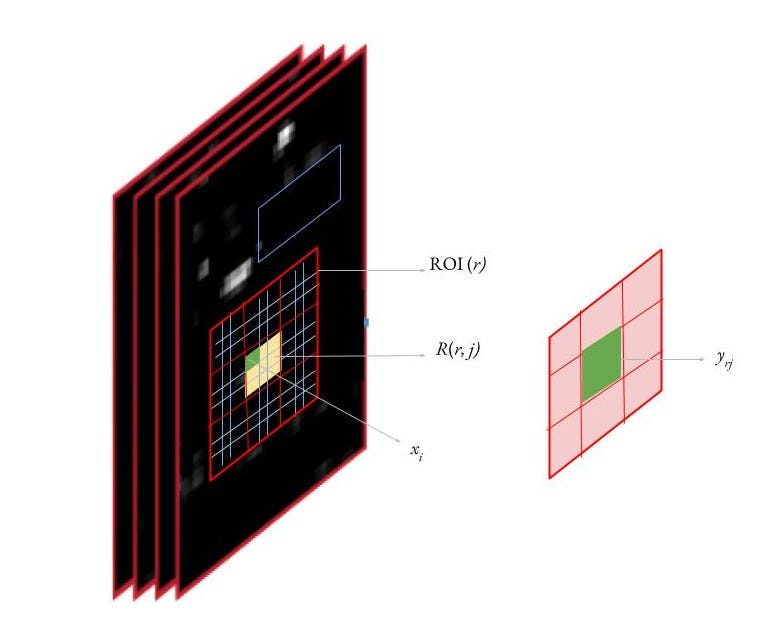
• Backpropagation through ROI pooling layer: For each mini-batch ROI r, let the ROI pooling output unit yᵣⱼ be the output of max-pooling in it’s sub-window R(r, j). Then, the gradient is accumulated in an input unit (xᵢ) in R(r, j) if this position i is the argmax selected for yᵣⱼ.

• In the multi-scale pipeline of Fast R-CNN, input images are resized into a randomly sampled size at train time to introduce scale invariance. At test time, each image is fed to the network in multiple fixed scales. For each ROI, the features are pooled from only one of these scales, chosen such that the scaled candidate window has the number of pixels closest to 224 x 224. However, the authors find that the single scale pipeline performs almost as well with a much lower computing time cost. In the single-scale approach, all images at train and test time are resized to 600 (shortest side) with the upper cap on the longest side being 1000.
• The large fully connected layers can be compressed with truncated SVD to make the network more efficient. Here a layer parameterized by W as its weight matrix can be factorized to reduce the parameter count by splitting it into two layers (ΣₜVᵀ and U with biases) without a non-linearity between them, where W ~ U ΣₜVᵀ.

Results

• Fast R-CNN achieved state of the art performance at the time of its publication on VOC12, VOC10(with additional data) and VOC07.
• Fast R-CNN processes images 45x faster than R-CNN at test time and 9x faster at train time. It also trains 2.7x faster and runs test images 7x faster than SPP-Net. On further using truncated SVD, the detection time of the network is reduced by more than 30% with just a 0.3 drop in mAP.
• Other contributions of the paper show that for larger networks fine-tuning the conv layers as well (and not just the FC layers like SPPnets) is really important to achieve significantly better mAP. For smaller networks, this improvement might not be as large.
• Multi-task training is not only easier but also improves performance because the tasks influence each other while training. Hence training the different stages of the network altogether improves it’s shared representative power (the backbone CNN)

This concludes the technical summary of the Fast R-CNN paper. Hope you enjoyed (understood)! 

References:

[1] Girshick, Ross et al. “Rich Feature Hierarchies for Accurate Object Detection and Semantic Segmentation.” 2014 IEEE Conference on Computer Vision and Pattern Recognition (2014)
[2] Girshick, Ross. “Fast R-CNN.” 2015 IEEE International Conference on Computer Vision (ICCV) (2015)
[3] He, Kaiming et al. “Spatial Pyramid Pooling in Deep Convolutional Networks for Visual Recognition.” Lecture Notes in Computer Science (2014)
[4] Uijlings, J. R. R. et al. “Selective Search for Object Recognition.” International Journal of Computer Vision 104.2 (2013)