R-CNN for object detection

In the rapidly growing field of deep learning, it is important to thoroughly understand some key concepts and milestones to develop skills beyond just using packages and toolboxes. Here is part of a series to understand the publications that are the fundamentals for current day object detection.

The original paper “Rich feature hierarchies for accurate object detection and semantic segmentation” [1] elaborates one of the first breakthroughs of the use of CNNs in an object detection system called the ‘R-CNN’ or ‘Regions with CNN’ which had a much higher object detection performance than other popular methods at the time.

Region proposals

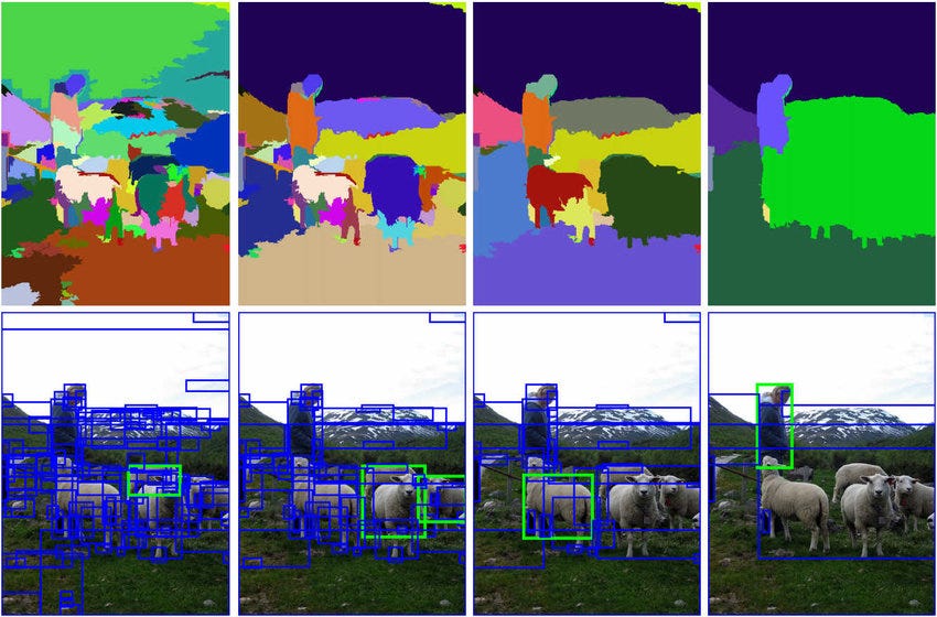
The first stage of the R-CNN pipeline is the generation of ‘region proposals’ or regions in an image that could belong to a particular object. The authors use the selective search algorithm. The selective search algorithm [2] works by generating sub-segmentations of the image that could belong to one object — based on color, texture, size and shape — and iteratively combining similar regions to form objects. This gives ‘object proposals’ of different scales. Note the R-CNN pipeline is agnostic to the region proposal algorithm. The authors use the selective search algorithm to generate 2000 category independent region proposals (usually indicated by rectangular regions or ‘bounding boxes’) for each individual image.

Figure 1: How the selective search algorithm iteratively obtains “region proposals”

Stage 1: Feature extraction from Region Proposals

At the end of this stage in the pipeline, the authors generate a 4096 dimensional feature vector from each of the 2000 region proposals for every image using a Convolutional Neural Network (CNN). The details of training this CNN are as given below.

Supervised Pre-training: The CNN described by Krizhevsky et al [3], now popularly known as the “AlexNet” has 5 convolutional and 2 fully connected layers. The CNN is first trained on the ILSVRC2012 classification dataset for a 1000 way image classification task with a large number of images so that the convolution layers can learn basic image features.

Domain-Specific Fine-Tuning: Now, the network needs to be fine-tuned to learn a) The visual features of the new types of images- distorted region proposals, and b) Specific target classes of the smaller dataset for the detection task. We fine-tune the classification network to identify the classes belonging to the detection task from the region proposals.

• The final 1000 way classification layer of the CNN from pre-training is replaced with a randomly initialized (N+1) way softmax classification layer for the N object classes and a general background class of the detection task.
• Inputs : Each of the 2000 region proposals generated from every image (using the selective search algorithm) are converted into fixed inputs of size 227 x 227 by a simple warping, irrespective of the size or aspect ratio to enable their use in fine-tuning the CNN (we need fixed-sized inputs irrespective of the actual dimensions to feed to the CNN). An additional parameter, p is used to indicate the amount of possible dilation of the original bounding box to include some context from the area around it.
• Labels for training: The authors map each object proposal to the ground-truth instance with which it has maximum IoU overlap and label it as a positive (for the matched ground-truth class) if the IoU is at least 0.5. The rest of the boxes are treated as the background class (negative for all classes).
• Training pipeline: The authors train the network using SGD with (1/10)th of the initial pre-training learning rate. In each iteration they sample 32 windows that are positive over all the classes and 96 windows that belong to the background class to form a mini-batch of 128, to ensure that there is enough representation from the positive classes during training.

Figure 2: The CNN training pipeline taking in a batch of region proposals and giving a classification label (at train time)

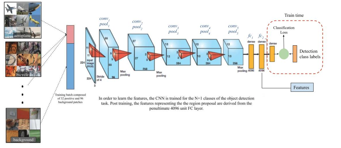
The final output of Stage 1: After training, the final classification layer is removed and a 4096 dimensional feature vector is obtained from the penultimate layer of the CNN for each of the 2000 region proposals (for every image). Refer to the image above.

Stage 2: SVM for object classification

This stage consists of learning an individual linear SVM (Support Vector Machine) classifier for each class, that detects the presence or absence of an object belonging to a particular class.

• Inputs: The 4096-d feature vector for each region proposal.
• Labels for training: The features of all region proposals that have an IoU overlap of less than 0.3 with the ground truth bounding box are considered negatives for that class during training. The positives for that class are simply the features from the ground truth bounding boxes itself. All other proposals (IoU overlap greater than 0.3, but not a ground truth bounding box) are ignored for the purpose of training the SVM.
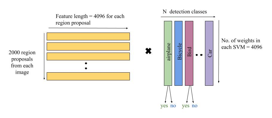
• Test time inference for a single image: The class-specific dot products between the features and SVM weights are consolidated into a single matrix-matrix product for an image (Figure 3 below). That is, for every image, a 2000 x 4096 feature matrix is generated (the 4096-d feature from the CNN for all 2000 region proposals). The SVM weight matrix is 4096 x N where N is the number of classes.

Figure 3: Final consolidated test time SVM computation

The final output of stage 2: After training the SVM, the final output of stage 2 is a set of positive object proposals for each class, from the CNN features of 2000 region proposals (of every image).

Stage 3: Bounding box regression

In order to improve localization performance, the authors include a bounding-box regression step to learn corrections in the predicted bounding box location and size.

Figure 4: The equations for bounding box regression stages explained below.

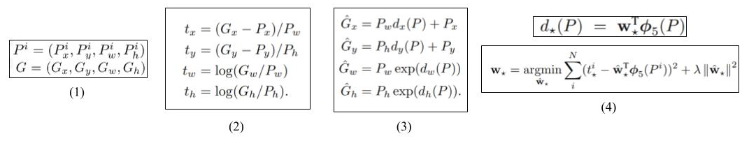
• Equation 1: The aim of this task is to learn a target transformation between our predicted proposal P and the target proposal G. The variables x, y, w, and h stand for the coordinates of the center (x, y) and the width w and height h of the proposal.
• Equation 2: The ground-truth transformations that need to be learnt are shown in equation 2. The first two transformations specify a scale-invariant translation of the center of P — x and y, and the second two specify log space transformations of the width w and height h.
• Equation 3: dₖ(P) where ₖ can belong to (x, y, h or w) is the predicted transformation. Ĝ signifies the corrected predicted box calculated using the original predicted box P and the predicted transformation dₖ(P).
• Equation 4: The predicted transformation dₖ(P) is modeled as a linear function of the pool₅(shown in Figure 2) features — Φ₅.
  Hence, dₖ(P) = wₖᵀ Φ₅(P) where wₖ is the vector of learnable model parameters. Note that Φ₅ is dependent on the actual image features. wₖ is learnt by optimizing the regularized least-squares objective function shown in the second line of equation 4.
• Other notes: The algorithm only learns from a predicted box P if it is near at least one groundtruth box. Each predicted box P is mapped to its groundtruth by choosing the groundtruth box with which it has a maximum overlap (provided it has an IoU overlap of at least 0.6). A separate transformation is learnt for each class of the detection task.

The final output of stage 3: For all the positive region proposals of each class predicted from the SVM, we have an accurate, corrected bounding box around the object.

Other Contributions

• At the time of it’s publication, the R-CNN achieved a mAP of 54% on PASCAL VOC 2010 and 31% on ILSVRC detection, much higher than its competing algorithms.
• One of the major other contributions of the paper was conclusive evidence that supervised pre-training for a similar task boosted performance much more than unsupervised pre-training.
• After a general analysis of the CNN, the authors found that without fine-tuning for the detection task, the network with the fully connected layers removed, was able to detect object proposals as well as the network with the fully connected layers attached — even though the former (pool₅) features are computed using only 6% of the network’s parameters. Post fine-tuning, the largest performance improvement occurred in the network including the FC layers. This showed that the convolutional layers contain more generalizable features than fully connected layers, which contain task-specific information.
• The authors hypothesize that the need for a separate SVM for detection rather than using the fine-tuned CNN itself for classification comes from a combination of several factors including a) The fact that the definition of positive examples used in fine-tuning does not emphasize precise localization and b) The softmax classifier in fine-tuning was trained on randomly sampled negative examples rather than on the subset of “hard negatives” used for SVM training.

References:

[1] Girshick, Ross et al. “Rich Feature Hierarchies for Accurate Object Detection and Semantic Segmentation.” 2014 IEEE Conference on Computer Vision and Pattern Recognition (2014)
[2] Uijlings, J. R. R. et al. “Selective Search for Object Recognition.” International Journal of Computer Vision 104.2 (2013)
[3] Alex Krizhevsky, Ilya Sutskever, Geoffrey E. Hinton “ImageNet Classification with Deep Convolutional Neural Networks”, Published in NIPS 2012