Faster R-CNN for object detection

The most widely used state of the art version of the R-CNN family — Faster R-CNN was first published in 2015. This article, the third and final one of a series to understand the fundamentals of current day object detection elaborates the technical details of the Faster R-CNN detection pipeline. For a review of its predecessors, check out these summaries: Regions with CNN (R-CNN) and Fast R-CNN.

In the R-CNN family of papers, the evolution between versions was usually in terms of computational efficiency (integrating the different training stages), reduction in test time, and improvement in performance (mAP). These networks usually consist of — a) A region proposal algorithm to generate “bounding boxes” or locations of possible objects in the image; b) A feature generation stage to obtain features of these objects, usually using a CNN; c) A classification layer to predict which class this object belongs to; and d) A regression layer to make the coordinates of the object bounding box more precise.

The only stand-alone portion of the network left in Fast R-CNN was the region proposal algorithm. Both R-CNN and Fast R-CNN use CPU based region proposal algorithms, Eg- the Selective search algorithm which takes around 2 seconds per image and runs on CPU computation. The Faster R-CNN [3] paper fixes this by using another convolutional network (the RPN) to generate the region proposals. This not only brings down the region proposal time from 2s to 10ms per image but also allows the region proposal stage to share layers with the following detection stages, causing an overall improvement in feature representation. In the rest of the article, “Faster R-CNN” usually refers to a detection pipeline that uses the RPN as a region proposal algorithm, and Fast R-CNN as a detector network.

Region Proposal Network (RPN)

Figure 1: The architecture of the region proposal network or RPN

Architecture

• The region proposal network (RPN) starts with the input image being fed into the backbone convolutional neural network. The input image is first resized such that it’s shortest side is 600px with the longer side not exceeding 1000px.
• The output features of the backbone network (indicated by H x W) are usually much smaller than the input image depending on the stride of the backbone network. For both the possible backbone networks used in the paper (VGG, ZF-Net) the network stride is 16. This means that two consecutive pixels in the backbone output features correspond to two points 16 pixels apart in the input image.
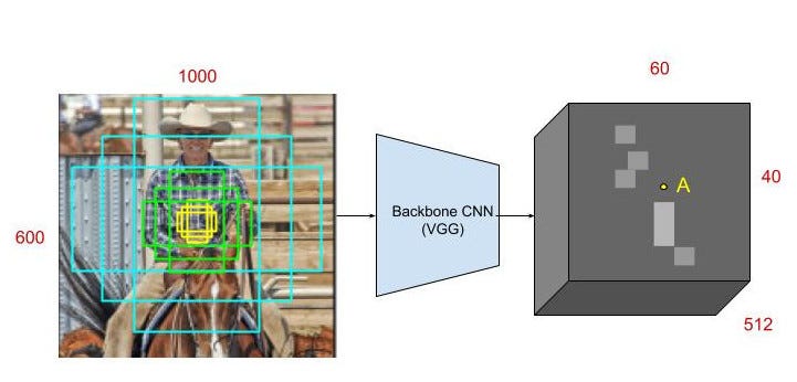
• For every point in the output feature map, the network has to learn whether an object is present in the input image at its corresponding location and estimate its size. This is done by placing a set of “Anchors” on the input image for each location on the output feature map from the backbone network. These anchors indicate possible objects in various sizes and aspect ratios at this location. The figure below shows 9 possible anchors in 3 different aspect ratios and 3 different sizes placed on the input image for a point A on the output feature map. For the PASCAL challenge, the anchors used have 3 scales of box area 128², 256², 512² and 3 aspect ratios of 1:1, 1:2 and 2:1.

Figure 2: The possible anchors in the input image in a location corresponding to point A in the feature map.

• As the network moves through each pixel in the output feature map, it has to check whether these k corresponding anchors spanning the input image actually contain objects, and refine these anchors’ coordinates to give bounding boxes as “Object proposals” or regions of interest.
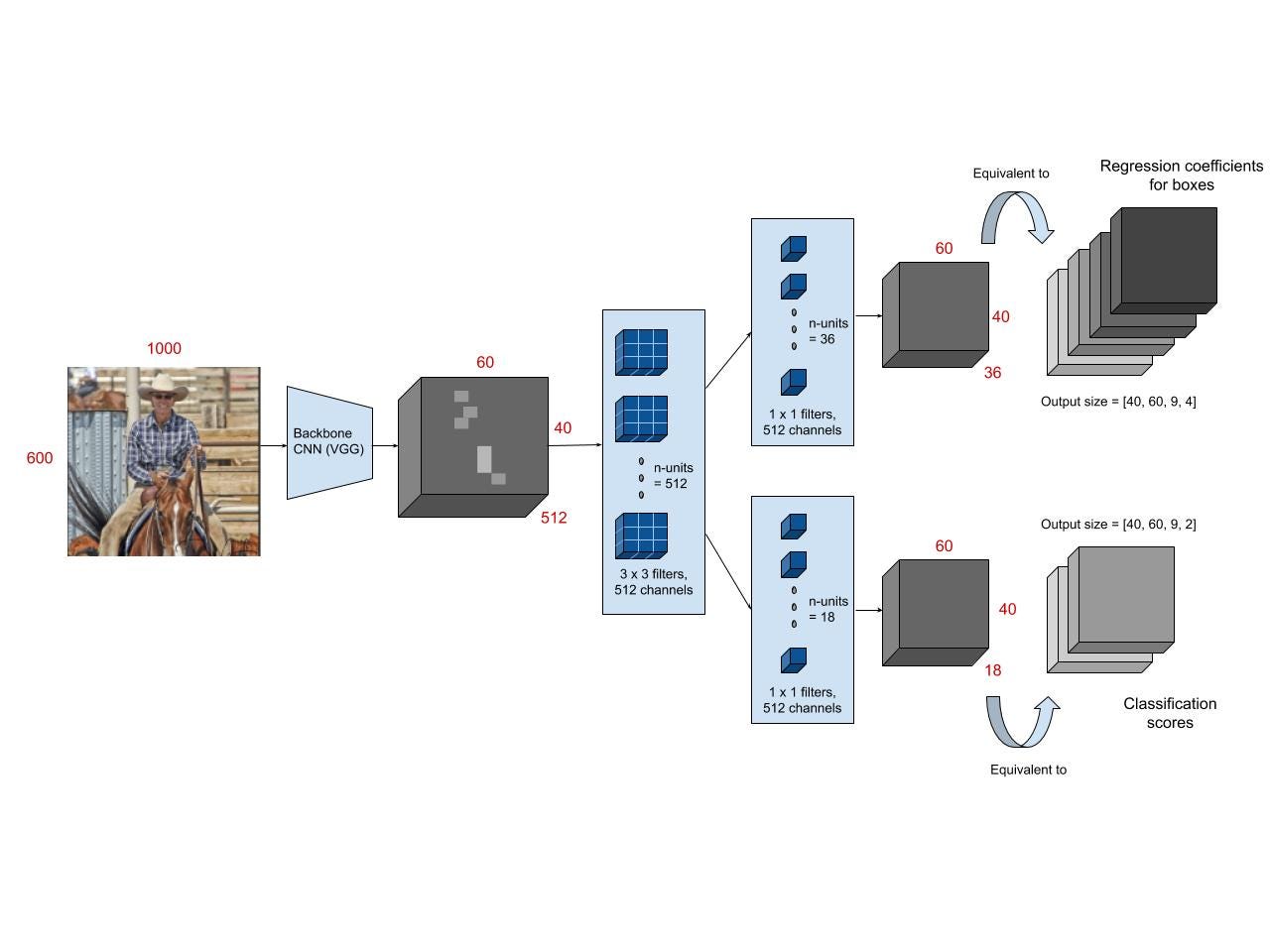
• First, a 3 x 3 convolution with 512 units is applied to the backbone feature map as shown in Figure 1, to give a 512-d feature map for every location. This is followed by two sibling layers: a 1 x 1 convolution layer with 18 units for object classification, and a 1 x 1 convolution with 36 units for bounding box regression.
• The 18 units in the classification branch give an output of size (H, W, 18). This output is used to give probabilities of whether or not each point in the backbone feature map (size: H x W) contains an object within all 9 of the anchors at that point.
• The 36 units in the regression branch give an output of size (H, W, 36). This output is used to give the 4 regression coefficients of each of the 9 anchors for every point in the backbone feature map (size: H x W). These regression coefficients are used to improve the coordinates of the anchors that contain objects.

Training and Loss functions

• The output feature map consists of about 40 x 60 locations, corresponding to 40*60*9 ~ 20k anchors in total. At train time, all the anchors that cross the boundary are ignored so that they do not contribute to the loss. This leaves about 6k anchors per image.
• An anchor is considered to be a “positive” sample if it satisfies either of the two conditions — a) The anchor has the highest IoU (Intersection over Union, a measure of overlap) with a groundtruth box; b) The anchor has an IoU greater than 0.7 with any groundtruth box. The same groundtruth box can cause multiple anchors to be assigned positive labels.
• An anchor is labeled “negative” if its IoU with all groundtruth boxes is less than 0.3. The remaining anchors (neither positive nor negative) are disregarded for RPN training.
• Each mini-batch for training the RPN comes from a single image. Sampling all the anchors from this image would bias the learning process toward negative samples, and so 128 positive and 128 negative samples are randomly selected to form the batch, padding with additional negative samples if there are an insufficient number of positives.
• The training loss for the RPN is also a multi-task loss, given by:

• Here i is the index of the anchor in the mini-batch. The classification loss L𝒸ₗₛ(pᵢ, pᵢ*) is the log loss over two classes (object vs not object). pᵢ is the output score from the classification branch for anchor i, and pᵢ* is the groundtruth label (1 or 0).
• The regression loss Lᵣₑ(tᵢ, tᵢ*) is activated only if the anchor actually contains an object i.e., the groundtruth pᵢ* is 1. The term tᵢ is the output prediction of the regression layer and consists of 4 variables [tₓ, tᵧ, tw, tₕ]. The regression target tᵢ* is calculated as —

• Here x, y, w, and h correspond to the (x, y) coordinates of the box centre and the height h and width w of the box. x*, xₐ stand for the coordinates of the anchor box and its corresponding groundtruth bounding box.
• Remember that all k (= 9) of the anchor boxes have different regressors that do not share weights. So the regression loss for an anchor i is applied to its corresponding regressor (if it is a positive sample).
• At test time, the learned regression output tᵢ can be applied to its corresponding anchor box (that is predicted positive), and the x, y, w, h parameters for the predicted object proposal bounding box can be back-calculated from —

Test time details

At test time, the 20k anchors from each image go through a series of post-processing steps to send in the object proposal bounding boxes.

• The regression coefficients are applied to the anchors for precise localization. This gives precise bounding boxes.
• All the boxes are arranged according to their cls scores. Then, a non-maximum suppression (NMS) is applied with a threshold of 0.7. From the top down, all of the bounding boxes which have an IoU of greater than 0.7 with another bounding box are discarded. Thus the highest-scoring bounding box is retained for a group of overlapping boxes.
• This gives about 2k proposals per image.
• The cross-boundary bounding boxes are retained and clipped to image boundary.
• While using these object proposals to train the Fast R-CNN detection pipeline, all 2k proposals from the RPN are used. At test time for Fast R-CNN detection, only the Top N proposals from the RPN are chosen.

Object detection: Faster R-CNN (RPN + Fast R-CNN)

Figure 3: The RPN for region proposals and Fast R-CNN as a detector in the Faster R-CNN detection pipeline

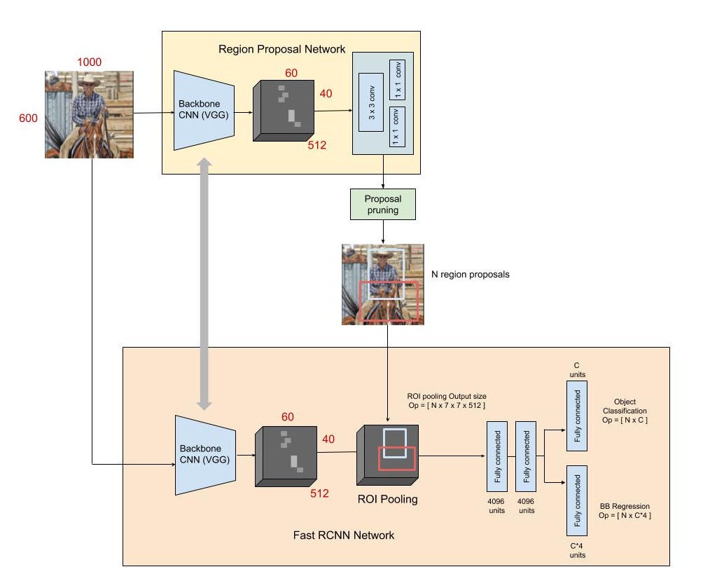
The Faster R-CNN architecture consists of the RPN as a region proposal algorithm and the Fast R-CNN as a detector network.

Fast R-CNN as a detector for Faster R-CNN

The Fast R-CNN detector also consists of a CNN backbone, an ROI pooling layer and fully connected layers followed by two sibling branches for classification and bounding box regression as shown in Figure 3.

• The input image is first passed through the backbone CNN to get the feature map (Feature size: 60, 40, 512). Besides test time efficiency, another key reason using an RPN as a proposal generator makes sense is the advantages of weight sharing between the RPN backbone and the Fast R-CNN detector backbone.
• Next, the bounding box proposals from the RPN are used to pool features from the backbone feature map. This is done by the ROI pooling layer. The ROI pooling layer, in essence, works by a) Taking the region corresponding to a proposal from the backbone feature map; b) Dividing this region into a fixed number of sub-windows; c) Performing max-pooling over these sub-windows to give a fixed size output. To understand the details of the ROI pooling layer and it’s advantages, read Fast R-CNN.
• The output from the ROI pooling layer has a size of (N, 7, 7, 512) where N is the number of proposals from the region proposal algorithm. After passing them through two fully connected layers, the features are fed into the sibling classification and regression branches.
• Note that these classification and detection branches are different from those of the RPN. Here the classification layer has C units for each of the classes in the detection task (including a catch-all background class). The features are passed through a softmax layer to get the classification scores — the probability of a proposal belonging to each class. The regression layer coefficients are used to improve the predicted bounding boxes. Here the regressor is size agnostic, (unlike the RPN) but is specific to each class. That is, all the classes have individual regressors with 4 parameters each corresponding to C*4 output units in the regression layer.
• For more details on how the Faster R-CNN is trained and its loss functions refer to Fast R-CNN.

4 Step Alternating training

In order to force the network to share the weights of the CNN backbone between the RPN and the detector, the authors use a 4 step training method:

a)The RPN is trained independently as described above. The backbone CNN for this task is initialized with weights from a network trained for an ImageNet classification task, and is then fine-tuned for the region proposal task.
b) The Fast R-CNN detector network is also trained independently. The backbone CNN for this task is initialized with weights from a network trained for an ImageNet classification task, and is then fine-tuned for the object detection task. The RPN weights are fixed and the proposals from the RPN are used to train the Faster R-CNN.
c) The RPN is now initialized with weights from this Faster R-CNN, and fine-tuned for the region proposal task. This time, weights in the common layers between the RPN and detector remain fixed, and only the layers unique to the RPN are fine-tuned. This is the final RPN.
d) Once again using the new RPN, the Fast R-CNN detector is fine-tuned. Again, only the layers unique to the detector network are fine-tuned and the common layer weights are fixed.

This gives a Faster R-CNN detection framework that has shared convolutional layers.

Figure 4: Results of the Faster R-CNN detection framework with a VGG backbone

Results

• In all the experiments on the PASCAL datasets, Fast R-CNN was chosen as a detector. The use of the RPN+ZF backbone as just a proposal network (without sharing weights with the detector) matched the performance of using “Selective Search” (SS) as a region proposal algorithm. This already gives us comparable results with a large decrease in detection time. RPN+VGG backbone as just a proposal network with unshared weights performs slightly better than the SS region proposal baseline. When using shared weights with the detector, both the ZF and VGG backbones in RPN surpassed the performance of the SS baseline. This along with a large number of other experiments validated the use of RPN as a region proposal method.
• Detection with a VGG RPN takes 198ms compared to the 1.8 seconds of Selective Search.
• The other experiments performed validate the use of NMS, and the use of separate classification and regression branches. The classification branch used to rank proposals by score seems to be an important factor in maintaining a reasonably high recall vs IoU overlap ratio even when the number of object proposals is reduced.
• In ablation studies to observe the importance of scale and aspect ratios of anchor boxes, the authors find that using 3 scales with a single aspect ratio works almost as well as 3 scales and 3 aspect ratios. Depending on the task and the dataset, these ratios and scales can be modified. Using a single anchor at each location causes the mAP to drop considerably.

This concludes the technical summary of the Faster R-CNN paper. Hope you enjoyed (understood)! 

References:

[1] Shaoqing Ren, Kaiming He, Ross Girshick, and Jian Sun, Faster R-CNN: Towards Real-Time Object Detection with Region Proposal Networks, NIPS’15 Proceedings
[2] http://www.telesens.co/2018/03/11/object-detection-and-classification-using-r-cnns/
[3] https://leonardoaraujosantos.gitbooks.io/artificial-inteligence/content/object_localization_and_detection.html