Comprehensive Guide to Convolutional Neural Networks

    A Convolutional Neural Network (ConvNet/CNN) is a Deep Learning algorithm that can take in an input image, assign importance (learnable weights and biases) to various aspects/objects in the image, and be able to differentiate one from the other. The pre-processing required in a ConvNet is much lower as compared to other classification algorithms. While in primitive methods filters are hand-engineered, with enough training, ConvNets have the ability to learn these filters/characteristics.

A ConvNet is able to successfully capture the Spatial and Temporal dependencies in an image through the application of relevant filters. The architecture performs a better fitting to the image dataset due to the reduction in the number of parameters involved and the reusability of weights. In other words, the network can be trained to understand the sophistication of the image better.

Convolution Layer — The Kernel

Image Dimensions = 5 (Height) x 5 (Breadth) x 1 (Number of channels, eg. RGB)

In the above demonstration, the green section resembles our 5x5x1 input image, I. The element involved in carrying out the convolution operation in the first part of a Convolutional Layer is called the Kernel/Filter, K, represented in the color yellow. We have selected K as a 3x3x1 matrix.

The Kernel shifts 9 times because of Stride Length = 1 (Non-Stride), every time performing a matrix multiplication operation between K and the portion P of the image over which the kernel is hovering.

The filter moves to the right with a certain Stride Value till it parses the complete width. Moving on, it hops down to the beginning (left) of the image with the same Stride Value and repeats the process until the entire image is traversed.

          Convolution operation on a MxNx3 image matrix with a 3x3x3 Kernel

The objective of the Convolution Operation is to extract the high-level features such as edges, from the input image. ConvNets need not be limited to only one Convolutional Layer. Conventionally, the first ConvLayer is responsible for capturing the Low-Level features such as edges, color, gradient orientation, etc. With added layers, the architecture adapts to the High-Level features as well, giving us a network which has the wholesome understanding of images in the dataset, similar to how we would.

There are two types of results to the operation — one in which the convolved feature is reduced in dimensionality as compared to the input, and the other in which the dimensionality is either increased or remains the same. This is done by applying Valid Padding in case of the former, or Same Padding in the case of the latter.

Pooling Layer

Similar to the Convolutional Layer, the Pooling layer is responsible for reducing the spatial size of the Convolved Feature. This is to decrease the computational power required to process the data through dimensionality reduction. Furthermore, it is useful for extracting dominant features which are rotational and positional invariant, thus maintaining the process of effectively training of the model.

                           3x3 pooling over 5x5 convolved feature

There are two types of Pooling: Max Pooling and Average Pooling. Max Pooling returns the maximum value from the portion of the image covered by the Kernel. On the other hand, Average Pooling returns the average of all the values from the portion of the image covered by the Kernel.

Max Pooling also performs as a Noise Suppressant. It discards the noisy activations altogether and also performs de-noising along with dimensionality reduction. On the other hand, Average Pooling simply performs dimensionality reduction as a noise suppressing mechanism. Hence, we can say that Max Pooling performs a lot better than Average Pooling.

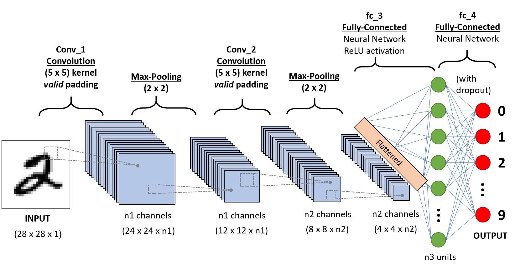
Classification — Fully Connected Layer (FC Layer)

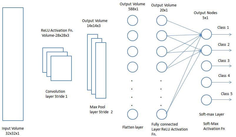
Adding a Fully-Connected layer is a (usually) cheap way of learning non-linear combinations of the high-level features as represented by the output of the convolutional layer. The Fully-Connected layer is learning a possibly non-linear function in that space.

Now that we have converted our input image into a suitable form for our Multi-Level Perceptron, we shall flatten the image into a column vector. The flattened output is fed to a feed-forward neural network and backpropagation applied to every iteration of training. Over a series of epochs, the model is able to distinguish between dominating and certain low-level features in images and classify them using the Softmax Classification technique.

There are various architectures of CNNs available which have been key in building algorithms which power and shall power AI as a whole in the foreseeable future. Some of them have been listed below:

1. LeNet
2. AlexNet
3. VGGNet
4. GoogLeNet
5. ResNet
6. ZFNet